The code below gives a simple implementation of the Metropolis and Metropolis-in-Gibbs sampling algorithms, which are useful for sampling probability densities for which the normalizing constant is difficult to calculate, are irregular, or have high dimension (Metropolis-in-Gibbs).
## Metropolis sampling
## x    - current value of Markov chain (numeric vector)
## targ - target log density function
## prop - function with prototype function(x, ...) that generates
##   a proposal value from a symmetric proposal distribution
library('mvtnorm')
prop_mvnorm <- function(x, ...)
  drop(rmvnorm(1, mean=x, ...))
metropolis <- function(x, targ, prop=prop_mvnorm, ...) {
  xnew <- prop(x)
  lrat <- targ(xnew, ...) - targ(x, ...)
  if(log(runif(1)) < lrat)
    x <- xnew
  return(x)
}

## Metropolis-in-Gibbs sampling
## x    - current value of Markov chain (numeric vector)
## targ - target log density function
## ...  - arguments passed to 'targ'
gibbs <- function(x, targ, ...) {
  for(i in 1:length(x)) {
    ## define full conditional
    targ1 <- function(x1, ...) {
      x[i] <- x1
      targ(x, ...)
    }
    ## sample using Metropolis algorithm
    x[i] <- metropolis(x[i], targ1, ...)
  }
  return(x)
}
The following code produces the figure below to illustrate the two methods using a 'dumbell' distribution (cf. R package 'ks' vignette).
### The code below illustrates the use of the functions above

## target 'dumbell' density (c.f., R package 'ks' vignette)
library('ks')
mus <- rbind(c(-2,2), c(0,0), c(2,-2))
sigmas <- rbind(diag(2), matrix(c(0.8, -0.72, -0.72, 0.8), nrow=2), diag(2))
cwt <- 3/11
props <- c((1-cwt)/2, cwt, (1-cwt)/2)
targ_test <- function(x, ...)
  log(dmvnorm.mixt(x, mus=mus, Sigmas=sigmas, props=props))

## plot contours of target 'dumbell' density
set.seed(42)
par(mfrow=c(1,2))
plotmixt(mus=mus, Sigmas=sigmas, props=props,
         xlim=c(-4,4), ylim=c(-4,4),
         xlab=expression(x[1]),
         ylab=expression(x[2]),
         main="Metropolis-in-Gibbs")

## initialize and sample using Metropolis-in-Gibbs
xcur <- gibbs(c(0,0), targ_test, sigma=vcov_test)
for(j in 1:2000) {
  xcur <- gibbs(xcur, targ_test, sigma=vcov_test)
  points(xcur[1], xcur[2], pch=20, col='#00000055')
}

## plot contours of target 'dumbell' density
plotmixt(mus=mus, Sigmas=sigmas, props=props,
         xlim=c(-4,4), ylim=c(-4,4),
         xlab=expression(x[1]),
         ylab=expression(x[2]),
         main="Metropolis")

## initialize and sample using Metropolis
xcur <- metropolis(c(0,0), targ_test, sigma=vcov_test)
for(j in 1:2000) {
  xcur <- metropolis(xcur, targ_test, sigma=vcov_test)
  points(xcur[1], xcur[2], pch=20, col='#00000055')
}
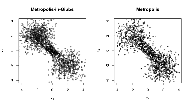
The figure illustrates two contrasting properties of the two methods:
- Metropolis-in-Gibbs samples can get 'stuck' in certain regions of the support, especially when there are multiple modes and/or significant correlation among the random variables. This is not as much a problem for Metropolis sampling.
- Metropolis sampling can produce fewer unique samples due to the poor approximation of the proposal density to the target density. This occurs more often for high-dimensional target densities.