I connected the instrumentation amplifier described in an earlier post to a piezoelectric transducer (buzzer) and made recordings at 5000 gain. The plot below shows 1000 such measurements over 1.0 seconds. There is a 4.0 second (at 1000Hz) sample of the data here piezo.csv. There is a clear sinusoidal signal in these data of about 60Hz. These findings were baffling at first, but apparently result from capacitative coupling between the measurement device and 60Hz household AC power lines.
I fit simple periodic mean model to these data:  , where
  is the measured ADC (Analog to Digital Converter) value,
  is time in seconds,
  is the mean ADC value,
  is the peak amplitude,
  is the frequency in Hertz,
  is the phase in radians, and
  is a zero-mean error term. The blue curve in the plot represents the least-squares fit to these data.

The least-squares estimates are as follows:
- - 577 ADC units
- - 7.75 ADC units
- - 59.9 Hz
- - 4.80 rad
The estimated frequency () is very close to the theoretical value (60). The ADC of the ATmega168 has 10 bit precision. That is, values can range from  to
to  . The Atmel manual gives the following formula for back-calculating the voltage at the ADC pin:
 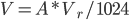 , where
  is the ADC value and
  is the reference voltage (
 in my setup). In addition, the instrumentation amplifier provides
  gain. Accounting for gain, the voltage measured between the instrumentation electrodes is
  . The estimated peak amplitude in ADC units was
  , so
, so  . That is, household AC coupling induced a
  peak potential between the instrumentation electrodes. In reality, the gain of the amplifier is less than
  , and is a lowball estimate.
Assuming there are no other signals in these data (which is likely incorrect), the residuals in this regression ought to resemble independent random variates. The histogram for the residuals looks good (bell shaped, no noticeable bias or skew), however, there is obvious residual autocorrelation. The figure below is a plot of the autocorrelation within the residuals.

It's clear that this method isn't quite ready to replace the pseudo-RNGs. As time permits, I plan to try some signal processing with these data, in hopes to isolate the independent noise. If the only signal is that induced by capacitative coupling, then a high pass filter (at 60Hz) ought to do the trick.
A recent blog post at Xi'An's mentioned some tests for randomness, including the Marsaglia Diehard Battery and the NIST Test Suite. Maybe if I get something that isn't obviously nonrandom, I'll try out some of these tests.
What about subsampling the signal to eliminate autocorrelation, much like is done is MCMC?
That's pretty cool!
Thanks Drew. It looks like the autocorrelation is periodic, like the signal. So, I'm afraid if I subsample at regular intervals, like thinning in MCMC, the autocorrelation would persist. Maybe subsampling at random intervals would improve the autocorrelation, but then that would require a [pseudo-]random number generator 🙂