Update 2019-12-07: A kind reader has pointed out that the quadrature points and weights returned by the hermite and gauss.hermite functions below (which are identical to those in the ecoreg and rmutil packages) are not a standard format. I have edited the post to use an alternate method to compute the Gauss-Hermite quadrature points and weights, using the gauss.quad function in the statmod package. Nevertheless, the results are identical in these examples below.
Statisticians often need to integrate some function with respect to the multivariate normal (Gaussian) distribution, for example, to compute the standard error of a statistic, or the likelihood function of a mixed effects model. In many (most?) useful cases, these integrals are intractable, and must be approximated using computational methods. Monte-Carlo integration is one such method; a stochastic method, but its computation can be prohibitively expensive, especially when the integral is computed many times.
Quadrature methods, which are deterministic rather than stochastic, are another set of methods that can be less computationally expensive, especially for lower-dimension integrals. The main idea is to approximate the integral as a weighted summation (the Monte-Carlo method uses an unweighted summation), where the integrand is evaluated on a grid of points selected from the domain of integration. The weights and points are carefully selected to approximate the integral. Gauss-Hermite quadrature is a well-known method for selecting the weights and points for integrals involving the univariate normal distribution. The details of selecting weights and points is complicated, and involves finding the roots of Hermite polynomials (see with Wikipedia link above for details). Fortunately, there already exists some R code (extracted from the ecoreg package; see the hermite and gauss.hermite functions below) that implements this.
There are natural extensions of univariate Gaussian quadrature for integrals involving the multivariate normal distribution. Peter Jäckel has written a great, short, accessible article about this, and some of the figures below look very similar to those in the article. The extension to multivariate integrals is based on the idea of creating an M-dimensional grid of points by expanding the univariate grid of Gauss-Hermite quadrature points, and then rotating, scaling, and translating those points according to the mean vector and variance-covariance matrix of the multivariate normal distribution over which the integral is calculated (see the mgauss.hermite function below, with comments). The weights of the M-variate quadrature points are the product of the corresponding M univariate weights. The following code block lists two functions, where the first computes the Gauss-Hermite quadrature weights and points in one dimension (using code from the statmod package), and the last computes the weights and points for multivariate Gaussian quadrature.
## perform quadrature of multivariate normal
library('statmod')
## Calculate nodes and weights for Gauss-Hermite quadrature
## with weights corresponding to standard normal distribution
gauss.hermite <- function(n) {
## Compute Gauss-Hermite quadrature nodes and weights
pts <- as.data.frame(gauss.quad(n, kind="hermite"))
## By default, the weight function for Hermite quadrature is
## w(x) = exp(-x^2). Need to adjust weights so that
## w(x) = (2*pi)^(1/2)*exp(-1/2*x^2)
pts$weights <- pts$weights * (2*pi)^(-1/2)*exp(pts$nodes^2/2)
## rename 'nodes' to comform with code below
pts$points <- pts$nodes
pts$nodes <- NULL
return(pts)
}
## compute multivariate Gaussian quadrature points
## n - number of points each dimension before pruning
## mu - mean vector
## sigma - covariance matrix
## prune - NULL - no pruning; [0-1] - fraction to prune
mgauss.hermite <- function(n, mu, sigma, prune=NULL) {
if(!all(dim(sigma) == length(mu)))
stop("mu and sigma have nonconformable dimensions")
dm <- length(mu)
gh <- gauss.hermite(n)
#idx grows exponentially in n and dm
idx <- as.matrix(expand.grid(rep(list(1:n),dm)))
pts <- matrix(gh$points[idx],nrow(idx),dm)
wts <- apply(matrix(gh$weights[idx],nrow(idx),dm), 1, prod)
## prune
if(!is.null(prune)) {
qwt <- quantile(wts, probs=prune)
pts <- pts[wts > qwt,]
wts <- wts[wts > qwt]
}
## rotate, scale, translate points
eig <- eigen(sigma)
rot <- eig$vectors %*% diag(sqrt(eig$values))
pts <- t(rot %*% t(pts) + mu)
return(list(points=pts, weights=wts))
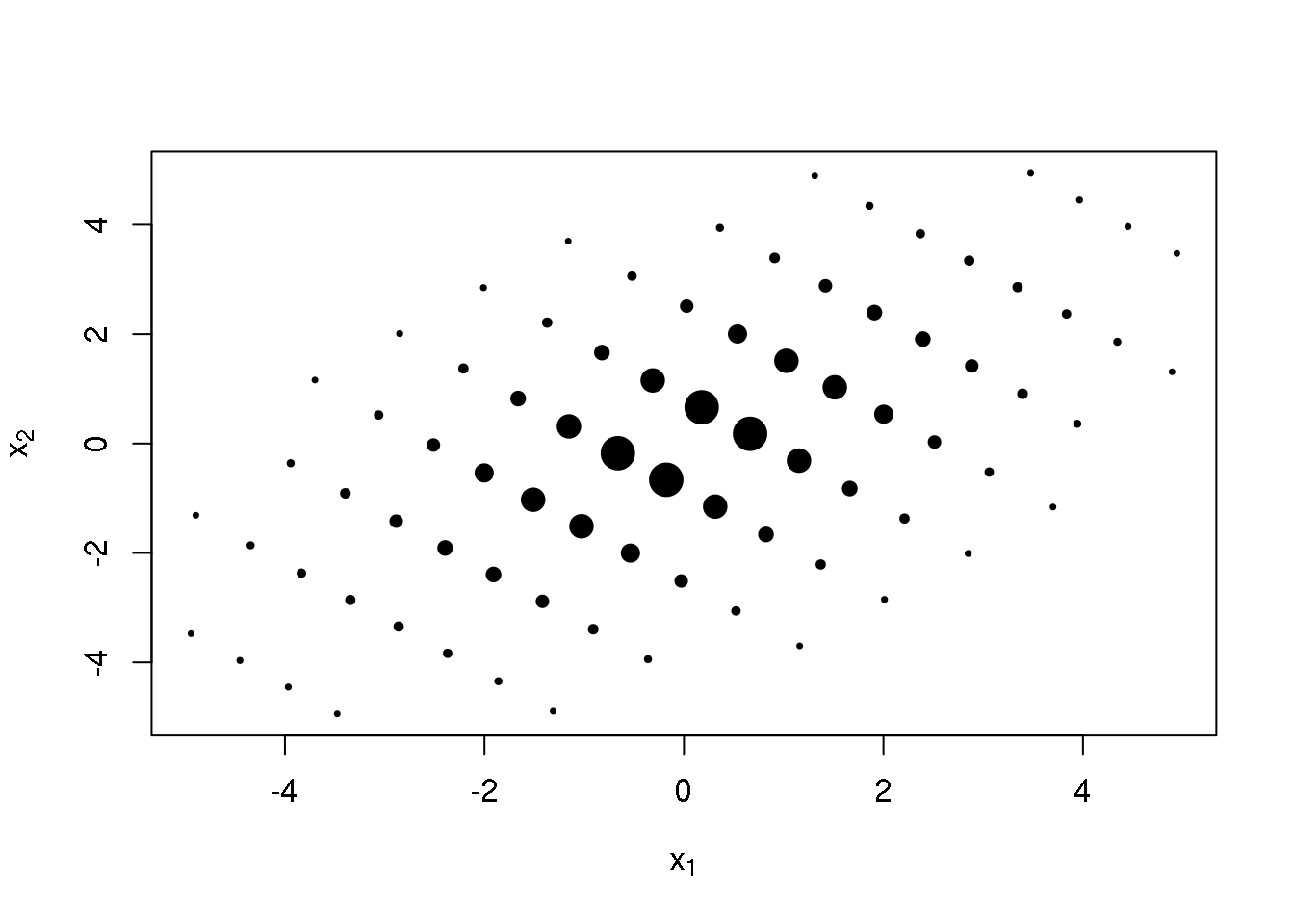
}For some of the M-variate points, the weights are very small, and thus contribute very little to the integral. The notion of ‘pruning’ can be used to eliminate those points with very small weights. The mgauss.hermite function does this by trimming a specified fraction of the smallest weights (I’ve found that pruning 20% often works well). In two dimensions, when the variance of each variable is 1.0 and correlation 0.5, the pruned points look as follows, where the point diameter is monotonic in the corresponding weight:
sig <- matrix(c(1,0.5,0.5,1),2,2)
pts <- mgauss.hermite(10, mu=c(0,0), sigma=sig, prune=0.2)
plot(pts$points, cex=-5/log(pts$weights), pch=19,
  xlab=expression(x[1]),
  ylab=expression(x[2]))
Computing a 2D integral with these points would require 80 evaluations of the integrand (note that there were originally 10 points in each dimension, or 100 points total, but by pruning were reduced to 80). Now, the real question is whether integrating with such points and weights can achieve a similar or better result than a same-sized (or perhaps even much larger) Monte-Carlo method. The following three sections compare these methods (and additionally the delta method, in the last section) in computing means and variances, probabilities, and the standard error of an unusual statistic. Probabilities are an interesting case because of the discreteness of the integrand, and computing standard errors is, obviously, an important application of quadrature.
Computing Means and Variance-Covariances
The true mean vector is zero, and the true variances and covariance are one and one-half, respectively. The quadrature method is the winner here:
library(mvtnorm); set.seed(42)
x80   <- rmvnorm(80, sigma=sig)
x1000 <- rmvnorm(1000, sigma=sig)

### Means
## quadrature with 80 points
colSums(pts$points * pts$weights)
## [1] -6.140989e-21  1.291725e-20

## Monte-Carlo with 80 points
colMeans(x80)
## [1] -0.06886731 -0.03477292

## Monte-Carlo with 1000 points
colMeans(x1000)
## [1] -0.02371047 -0.01133503

### Variances
## quadrature with 80 points
cov.wt(pts$points, wt=pts$weights, method="ML")$cov
##           [,1]      [,2]
## [1,] 0.9999904 0.4999952
## [2,] 0.4999952 0.9999904

## Monte-Carlo with 80 points
cov(x80)
##           [,1]      [,2]
## [1,] 0.9838169 0.4958186
## [2,] 0.4958186 1.0174029

## Monte-Carlo with 1000 points
cov(x1000)
##           [,1]      [,2]
## [1,] 1.0083872 0.4938198
## [2,] 0.4938198 0.9727271
Computing Probabilities
Computing probabilities is the same as using an indicator functions as the integrand in this context, which are obviously much more discrete than the integrand for means. It looks like the Monte-Carlo methods may be superior in computing such quantities. For the first probability, the true value is 1/3; for the second, the true value is 1/20:
### Probabilities
## P(x1<0, x2<0) = 1/3
## quadrature with 80 points
gfun <- function(x) prod(x<0)
sum(apply(pts$points, 1, gfun) * pts$weights)
## [1] 0.3927074

## Monte-Carlo with 80 points
mean(apply(x80, 1, gfun))
## [1] 0.3625

## Monte-Carlo with 1000 points
mean(apply(x1000, 1, gfun))
## [1] 0.336

## P(x1<q0.05, x2<q0.05) = 0.05
q0.05 <- qmvnorm(0.05, sigma=sig)$quantile
gfun  <- function(x) prod(x<q0.05)
## quadrature with 80 points
sum(apply(pts$points, 1, gfun) * pts$weights)
## [1] 0.01911414

## Monte-Carlo with 80 points
mean(apply(x80, 1, gfun))
## [1] 0.0625

## Monte-Carlo with 1000 points
mean(apply(x1000, 1, gfun))
## [1] 0.06
Computing Standard Errors for Unusual Statistics
Consider a model described by a vector of parameters, and an estimator that has an approximate multivariate normal distribution. This is often the case, for example, with ordinary least-squares and maximum likelihood estimators.
As an example, consider the one-compartment pharmacokinetic model with first-order elimination and intravenous bolus injection. The cfun function below gives the concentration of drug as a function of time following an IV bolus. The tfun function computes the time at which the concentration reaches a given level. As our statistic of interest, consider the amount of time in which the concentration remains above 0.064 g/L, which is four-fold the typical minimum inhibitory concentration (MIC) of piperacillin, an antibiotic. The figure below illustrates the time-course of piperacillin concentration for a typical patient after a 3g IV bolus.
## drug concentration after bolus injection
## one-compartment model
cfun <- function(t,v,k,dose=3)
  dose/v*exp(-k*t)

## compute time at which concentration reaches x
tfun <- function(x,v,k,dose=3)
  -log(x*v/dose)/k

## compute time at which concentration reaches 0.064
## given parameters p=c(v,k)
gfun <- function(p)
  tfun(0.064, p[1], p[2])

## from a recent PK study on piperacillin
log_mu  <- c(log_v=3.444, log_k=-2.036)
log_sig <- structure(c(0.0033, -0.0022, -0.0022, 0.0034),
            .Dimnames = rep(list(c("log_v", "log_k")),2),
            .Dim = c(2L, 2L))

curve(cfun(x, v=exp(log_mu[1]), k=exp(log_mu[2])),
      from=0, to=8, n=300,
      xlab="Time (h)", ylab="Concentration (g/L)")
lines(x=c(-10,rep(gfun(exp(log_mu)),2)),
      y=c(rep(0.064,2), 0), lty=2)
legend("topright", bty="n",
  legend=paste0("Time to 0.064 g/L: ",
    round(gfun(exp(log_mu)),1), "h"))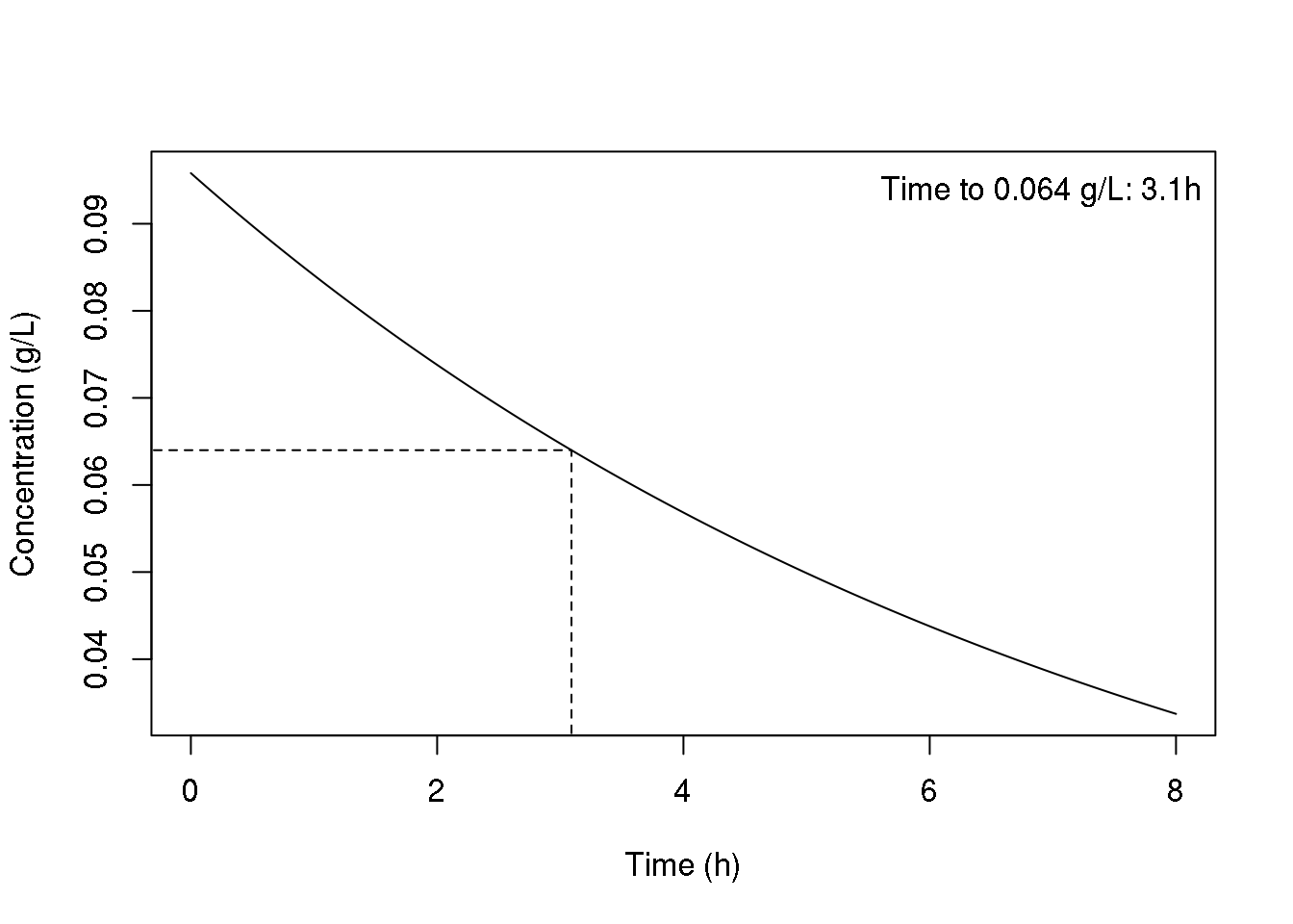
Since the amount of time in which the concentration remains above 0.064 g/L is a function of the model parameters, sampling variability in the parameter estimates propagate, and thus we can compute a standard error. The "true" standard error is approximately 0.1233, which was computed (ironically) using the Monte Carlo method with 10M sample points. Below, the standard error is approximated using quadrature with 80 points, Monte Carlo with 80 and 1000 points, and the delta method. Each of the methods perform fairly well here. However, this is a fairly 'smooth' statistic. In fact, my motivation for this little experiment is to lay the groundwork to examine a more complex statistic: the probabilities of pharmacokinetic target attainment in a population. These statistics are usually calculated using a Monte Carlo method ("Monte Carlo Simulation" or MCS, in the antibiotic literature), and are thus somewhat discrete. That is, even for large MCSs, the numerical delta method (i.e., where the gradient is computed numerically) can fail miserably.
## quadrature with 80 points
pts <- mgauss.hermite(n=10, mu=log_mu, sigma=log_sig, prune=0.2)
cov.wt(matrix(apply(exp(pts$points), 1, gfun), nrow(pts$points),1),
       pts$weights, method="ML")$cov
##           [,1]
## [1,] 0.1232139

## Monte-Carlo with 80 points
var(apply(exp(rmvnorm(80, mean=log_mu, sigma=log_sig)), 1, gfun))
## [1] 0.123917

## Monte-Carlo with 1000 points
var(apply(exp(rmvnorm(1e3, mean=log_mu, sigma=log_sig)), 1, gfun))
## [1] 0.1219701

## delta method
rho <- list2env(list(log_v=log_mu[1],log_k=log_mu[2],x=0.064))
nd <- attr(numericDeriv(quote(tfun(x,exp(log_v),exp(log_k))),
           theta=c('log_v','log_k'),rho=rho), 'gradient')
nd %*% log_sig %*% t(nd)
##          [,1]
## [1,] 0.121936