I recently decided to revisit some R code that implements a Gibbs sampler in an attempt to decrease the iteration time. My strategy was to implement the sampler state as an R environment rather than a list. The rationale was that passing an environment to and from functions would reduce the amount of duplication (memory copying). In my experiments, this results in only marginal improvement in iteration time. The following is just a toy example to illustrate.
Consider the logistic regression model
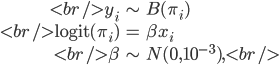
where
 is a binary outcome, independently Bernoulli distributed with probability
  ,
,  is a scalar covariate, and the log odds
  is a priori normal distributed with mean
  and precision
  .
.
For Gibbs sampling, it's convenient to store and manupulate a model state. In the past, I had represented this in R with a list, for example
> logit <- function(e) log(e) - log(1-e)
> expit <- function(l) exp(l) / (1+exp(l))
> # Simulate some data
> n <- 1e3
> x <- runif(n)
> y <- rbinom(n, 1, expit(5*x))
> iter <- 0
> itermax <- 1000
> state <- list(x=x, y=y, mu=0, tau=1e-3, beta=rep(0,itermax), iter=1)
Then, to perform a Gibbs update on beta, I would pass the old state to a function that would return the updated state. For example:
> Gibbs <- function(state) {
+     # Metropolis update
+     state$iter <- state$iter + 1
+
+     old_beta  <- state$beta[state$iter-1]
+     old_probs <- expit(old_beta*state$x)
+     old_logp  <- sum(log(ifelse(state$y,old_probs,1-old_probs))) +
+                  dnorm(old_beta, state$mu, 1/sqrt(state$tau), log=TRUE)
+
+     new_beta  <- rnorm(1, old_beta) # Proposal
+     new_probs <- expit(new_beta*state$x)
+     new_logp  <- sum(log(ifelse(state$y,new_probs,1-new_probs))) +
+                  dnorm(new_beta, state$mu, 1/sqrt(state$tau), log=TRUE)
+
+     if(new_logp - old_logp > log(runif(1)))
+         state$beta[state$iter] <- new_beta
+     else
+         state$beta[state$iter] <- old_beta
+
+     return(state)
+ }
Hence, the Gibbs sampler would be used as follows
> system.time({
+ while(state$iter < itermax)
+     state <- Gibbs(state)
+ })
   user  system elapsed
  2.708   0.012   2.717
> summary(state$beta)
   Min. 1st Qu.  Median    Mean 3rd Qu.    Max.
  0.000   4.414   4.564   4.515   4.792   5.417
Alternatively, the Gibbs sampler state may be stored and manipulated asan R environment. For example, to initialize the state:
> estate <- new.env()
> assign("x", x, envir=estate)
> assign("y", y, envir=estate)
> assign("mu", 0, envir=estate)
> assign("tau", 1e-3, envir=estate)
> assign("beta", rep(0,itermax), envir=estate)
> assign("iter", 1, envir=estate)
Then rewrite the Gibbs sampler function:
> GibbsExp <- expression({
+     # Metropolis update
+     iter <- iter + 1
+
+     old_beta  <- beta[iter-1]
+     old_probs <- expit(old_beta*x)
+     old_logp  <- sum(log(ifelse(y,old_probs,1-old_probs))) +
+                  dnorm(old_beta, mu, 1/sqrt(tau), log=TRUE)
+
+     new_beta  <- rnorm(1, old_beta) # Proposal
+     new_probs <- expit(new_beta*x)
+     new_logp  <- sum(log(ifelse(y,new_probs,1-new_probs))) +
+                  dnorm(new_beta, mu, 1/sqrt(tau), log=TRUE)
+
+     if(new_logp - old_logp > log(runif(1)))
+         beta[iter] <- new_beta
+     else
+         beta[iter] <- old_beta
+ })
>
> eGibbs <- function(estate) {
+     eval(GibbsExp, estate)
+ }
The Gibbs sampler is used in an almost identical manner:
> system.time({
+ while(get("iter",envir=estate) < itermax)
+     eGibbs(estate)
+ })
   user  system elapsed
  2.664   0.000   2.673
> summary(get("beta",envir=estate))
   Min. 1st Qu.  Median    Mean 3rd Qu.    Max.
  0.000   4.378   4.588   4.556   4.779   5.704
The percent decrease in iteration time is fairly constant for a variety of n and maxiter values. Presumably, this modest gain in speed results from less memory duplication. However, in some experiments with tracemem the story appears to be more complicated... For now, it doesn't appear that utilizing environments is worth the trouble when the sampling algorithm is much slower than memory allocation.
Thanks for this Matt. How about using the proto package rather than environments directly ? It probably won't make any difference to the running time but the semantic sugar is nice
In case it's of interest, here is your example reworked to use prototypes (proto package) rather than simple R environments.
library(proto) Gibbs <- proto() Gibbs$new <- function(., x, y) { proto(., x=x, y=y) } Gibbs$run <- function(., niter, adapt=0, mu=0, tau=0.001) { .$beta <- numeric(niter) .$mu <- mu .$tau <- tau beta.old <- 0 for (i in 1:adapt) { beta.old <- .$update(beta.old) } for (i in 1:niter) { beta.old <- .$update(beta.old) .$beta[i] <- beta.old } } Gibbs$update <- function(., beta.old) { probs.old <- plogis(beta.old * .$x) logp.old <- sum( log( ifelse(.$y , probs.old, 1-probs.old) ) ) + dnorm(beta.old, .$mu, 1/sqrt(.$tau), log=TRUE) beta.new <- rnorm(1, beta.old) # Proposal probs <- plogis(beta.new * .$x) logp <- sum( log( ifelse( .$y, probs, 1 - probs ) ) ) + dnorm(beta.new, .$mu, 1/sqrt(.$tau), log=TRUE) ifelse (logp - logp.old > log(runif(1)), beta.new, beta.old) } #Using the sampler x <- rnorm(1000) y <- rbinom(1000, 1, plogis(5*x)) gibbs <- Gibbs$new(x, y) gibbs$run(5000) summary(gibbs$beta) Min. 1st Qu. Median Mean 3rd Qu. Max. 0.5253 5.1030 5.3480 5.3570 5.6130 6.7160Which seems to be slower than the previous two solutions - I run it several times and timings were quite consistent.
> system.time(gibbs$run(1000))
user system elapsed
3.19 0.00 3.19
Yes, it quite probably is slower. I wasn't suggesting proto for speed but for neat encapsulation. However, after posting the code I realized that there is an obvious improvement to be made that might reduce run time: rather than calculate probs.old and logp.old on each update, simply store the previous logp value. For example...
Michael, previously I did not looked at the maths of your implementation, but the results do not match with Matt. In addition, your R code in the last post is incomplete.
Sorry Gregor, I forgot to escape characters for html. Here is the code again...
When I've run this with the same example that Matt uses I get a good recovery of the coefficient value (mean posterior) but I haven't checked to see the posterior density is different in other respects. I'll do that.
Oh dear, didn't escape the characters properly 🙁 I'll try again shortly
Hopefully this one works...
Gibbs$update <- function(., beta.old) {
  beta.new <- rnorm(1, beta.old) # Proposal
  probs <- plogis(beta.new * .$x)
  logp <- sum( log( ifelse( .$y, probs, 1 - probs ) ) ) +
          dnorm(beta.new, .$mu, 1/sqrt(.$tau), log=TRUE)

  if (logp - .$logp.old > log(runif(1))) {
    .$logp.old <- logp
    return( beta.new )
  } else {
    return( beta.old )
  }
}