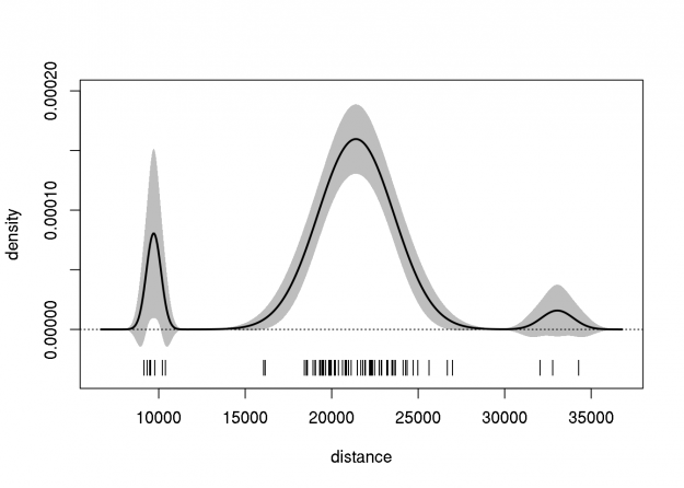
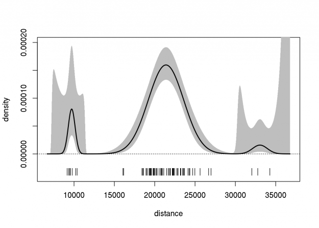
This post follows from a previous post (2798), in which the delta method was used to create an approximate pointwise 95% confidence band for a Gaussian density estimate. Note that the quality of this estimate was not assessed (e.g., whether the band has the correct pointwise coverage). Here we extend that approach to the Gaussian mixture density, which is much more flexible, and given sufficient mixture components, can be used to model ANY density. Here we show how the delta method can behave badly...

The parameters of mixture distributions are difficult to estimate by directly optimizing the likelihood function, because there are multiple constraints on the parameter space, and because the likelihood function is a sum. To overcome this, we most often use the EM algorithm. In the code below, I use the normalmixEM function from the mixtools package to estimate the parameters of a three-component Gaussian mixture, fitted to the famous galaxies data from the MASS package. Then, I compute the numerical Hessian of the log likelihood function to approximate the sampling variance-covariance of the parameter estimates. The remaining steps are the familiar delta method.

library("MASS") ## galaxies data
library("mixtools") ## normalmixEM
library("nlme") ## fdHess

## log likelihood function
llik <- function(x, mu, sig, lam) {
  if(any(lam==0)||any(lam==1)||any(sig<0))
    return(-sqrt(.Machine$double.xmax))
  sum(sapply(x, function(y)
    log(sum(dnorm(y, mu, sig)*lam))))
}

## convenience log likelihood function
llikp <- function(par, x=galaxies)
  llik(x,par[1:3],par[4:6],c(par[7:8],1-sum(par[7:8])))

## mixture density function
mixdens <- function(par, x=galaxies)
  t(sapply(x, function(y)
    sum(dnorm(y, par[1:3], par[4:6])*
          c(par[7:8],1-sum(par[7:8])))))

## log of mixture density function
lmixdens <- function(par, x=galaxies)
  log(mixdens(par, x))

## compute the finite-difference gradient (c.f., nlme::fdHess)
fdGrad <- function (pars, fun, ...,
                    .relStep = (.Machine$double.eps)^(1/3), 
          minAbsPar = 0) {
  pars <- as.numeric(pars)
  npar <- length(pars)
  incr <- ifelse(abs(pars) <= minAbsPar, minAbsPar * .relStep, 
                 abs(pars) * .relStep)
  ival <- do.call(fun, list(pars, ...))
  diff <- rep(0,npar)
  sapply(1:npar, function(i) {
    del <- rep(0,npar)
    del[i] <- incr[i]
    (do.call(fun, list(pars+del, ...))-ival)/incr[i]
  })
}

## fit three-component normal mixture to galaxies data
set.seed(42)
pars <- normalmixEM(galaxies, k=3,
  mu=quantile(galaxies, probs=c(0,1/2,1)))

## extract parameter estimates
pars <- c(pars$mu, pars$sigma, pars$lambda[1:2])

## compute Hessian of log likelihood function
hess <- fdHess(pars, llikp)$Hessian

## compute approximate var-cov of estimates
vcov <- solve(-hess)

## delta method to approximate var-cov of density 
grng <- extendrange(galaxies, f=0.10)
grid <- seq(grng[1], grng[2], length.out=500)
dgrd <- fdGrad(pars, mixdens, x=grid)
dvar <- dgrd %*% vcov %*% t(dgrd)
mden <- mixdens(pars, grid)

## plot density and confidence bands
plot(grid, mden, ylim=extendrange(mden,f=0.25), type="l",
     xlab="distance", ylab="density")
polygon(c(grid, rev(grid)), 
        c(mden + qnorm(0.975)*sqrt(diag(dvar)),
          rev(mden - qnorm(0.975)*sqrt(diag(dvar)))),
        col="gray", border=NA)
lines(grid, mden, lwd=2)
abline(h=0, lty=3)

## rug plot of galaxies data
points(galaxies, rep(par("usr")[3]+diff(par("usr")[3:4])/15,
                     length(galaxies)), pch="|")

On first glance, this confidence band is less than satisfactory because the lower bound is less than zero in some places. In order to fix this, I tried using the delta method on the logarithm of the mixture density estimate (similar to how we compute confidence intervals for odds ratios). This does indeed force the confidence limits to be positive. However, the upper limits are strange.

## recompute using log of mixture density
ldgrd <- fdGrad(pars, lmixdens, x=grid)
ldvar <- ldgrd %*% vcov %*% t(ldgrd)
lmden <- lmixdens(pars, grid)

## plot density and confidence bands
plot(grid, exp(lmden), ylim=extendrange(exp(lmden),f=0.25),
     type="l", xlab="distance", ylab="density")
polygon(c(grid, rev(grid)), 
        exp(c(lmden + qnorm(0.975)*sqrt(diag(ldvar)),
          rev(lmden - qnorm(0.975)*sqrt(diag(ldvar))))),
        col="gray", border=NA)
lines(grid, exp(lmden), lwd=2)
abline(h=0, lty=3)

## rug plot of galaxies data
points(galaxies, rep(par("usr")[3]+diff(par("usr")[3:4])/15,
                     length(galaxies)), pch="|")

Finally, I should mention that neither of these confidence bands may be any good. Ideally, these intervals would be assessed using a simulation (or perhaps a nonparametric bootstrap) to check their quality.