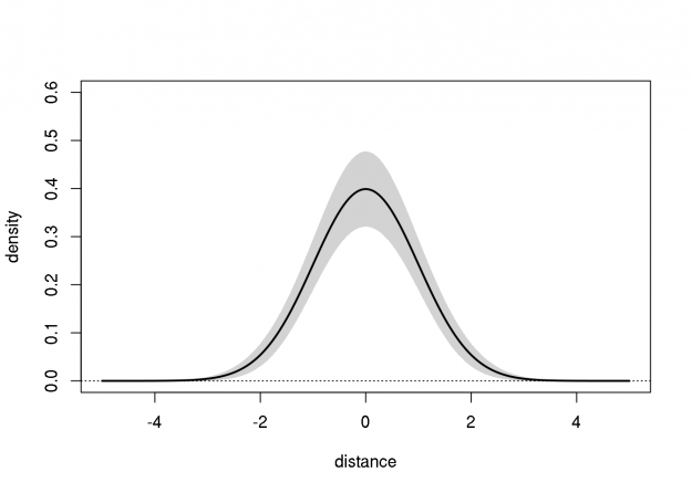
During one of our Department's weekly biostatistics "clinics", a visitor was interested in creating confidence bands for a Gaussian density estimate (or a Gaussian mixture density estimate). The mean, variance, and two "nuisance" parameters, were simultaneously estimated using least-squares. Thus, the approximate sampling variance-covariance matrix (4x4) was readily available. The two nuisance parameters do not directly affect the Gaussian density, but the client was concerned that their correlation with the mean and variance estimates would affect the variance of the density estimate. Of course, this might be the case in general, and a nonparametric bootstrap method might be used to account for this. Nevertheless, I proposed using the delta method, in which the variability of the nuisance parameter estimates do not affect that of the density estimate; a consequence of the normality assumption. This can be verified by fiddling with the parameters below.
The code below implements a Wald-type pointwise 95% confidence band for a test case; I made up the values of the estimated parameters and their approximate variance-covariance matrix (note that the mean and variance estimators are statistically independent). After fiddling with this a bit, it's clear that this delta method approach can perform poorly when the sampling variance is large (e.g., the lower bound of the density estimate can be negative).
## bell curve function
bell <- function(dist, mu=0, sig=1, p1=0, p2=0)
  exp(-(dist-mu)^2/sig/2)/sqrt(2*pi)/sig

## plot bell curve at default parameters
curve(bell(x), from=-5, to=5, ylim=c(0,0.6),
      ylab="density", xlab="distance")

## compute gradient of bell_curve on a grid of distances
dgrid <- seq(-5, 5, 1/50)
bderv <- numericDeriv(
  expr=quote(bell(dgrid, mu, sig, p1, p2)),
  theta=c("mu","sig","p1","p2"),
  rho=list2env(list(dgrid=dgrid,mu=0,sig=1,p1=0,p2=0)))
bgrad <- attr(bderv, 'gradient')

## variance-covariance matrix of mu, sig, p1, and p2
pvcov <- matrix(c(1.0,0.0,0.1,0.0,
                  0.0,1.0,0.0,0.1,
                  0.1,0.0,0.2,0.1,
                  0.0,0.1,0.1,0.2)/100, 4,4)

## approxiamte variance-covariance of bell curve
## induced by variability in parameters
bvcov <- bgrad %*% pvcov %*% t(bgrad)

## add pointwise 95% Wald confidence bands
polygon(x=c(dgrid, rev(dgrid)),
        y=c(bderv + qnorm(0.975)*sqrt(diag(bvcov)),
            bderv - qnorm(0.975)*sqrt(diag(bvcov))),
        col="lightgray", border=NA)
lines(dgrid, bderv, lwd=2)
abline(h=0, lty=3)
