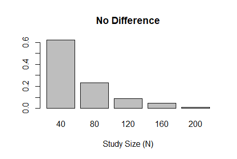
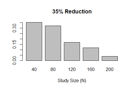
I had an opportunity recently to design a Bayesian adaptive trial with several interim analyses that allow for early stopping due to efficacy or futility. The code below implements the one-arm, binary outcome trial described in the great introductory article by Ben Saville et al. Three of the coauthors are current or former colleagues at Vandy. Assessment of trial efficacy (at interim and final analyses) is determined using posterior probabilities. However, futility is assessed using posterior predictive probability; the probability of concluding efficacy if the trial continues to the maximum sample size. In this example, the outcome is modeled using the binomial distribution, where the outcome probability has a uniform (beta) prior distribution; a conjugate prior. This makes the posterior (also beta) and posterior predictive (beta-binomial) probabilities easy to calculate. The figures below the code show the sample size distribution under the null hypothesis and an alternative hypothesis, respectively.
## Simulate Bayesian single-arm adaptive trial
## Allow early termination due to futility or efficacy
## Binary outcome
## Beta-binomial:
##   p   ~ beta(a, b)
##   x_i ~ binomial(p)  i = 1..n
##   p|x ~ beta(a + sum(x), b + n - sum(x))
## Efficacy at interim t if Pr(p > p_0 | x_{(t)}) > \gamma_e
## Futility at interim t if Pr(p > p_0 | x_{(t_max)}) < \gamma_f
## https://www.ncbi.nlm.nih.gov/pmc/articles/PMC4247348/

library('rmutil') ## for betabinom
## Simulate entire trial
## ptru - true probability of outcome (p)
## pref - reference probability of outcome (p_0)
## nint - sample sizes at which to conduct interim analyses
## efft - efficacy threshold
## futt - futility threshold
## apri - prior beta parameter \alpha
## bpri - prior beta parameter \beta
simtrial <- function(
  ptru = 0.15,
  pref = 0.15,
  nint = c(10, 13, 16, 19),
  efft = 0.95,
  futt = 0.05,
  apri = 1,
  bpri = 1) {

  ## determine minimum number of 'successes' necessary to
  ## conclude efficacy if study continues to maximum
  ## sample size
  nmax <- max(nint)
  post <- sapply(0:nmax, function(nevt)
    1-pbeta(pref, apri + nevt, bpri + nmax - nevt))
  nsuc <- min(which(post > efft)-1)


  ## simulate samples
  samp <- rbinom(n = nmax, size = 1, prob = ptru)

  ## simulate interim analyses
  intr <- lapply(nint, function(ncur) {

    ## compute number of current events
    ecur <- sum(samp[1:ncur])

    ## compute posterior beta parameters
    abb <- apri + ecur
    bbb <- bpri + ncur - ecur
    sbb <- abb + bbb
    mbb <- abb/(abb+bbb)

    ## compute efficacy Pr(p > p_0 | x_{(t)})
    effp <- 1-pbeta(pref, abb, bbb)

    ## return for efficacy
    if(effp > efft)
      return(list(action='stop',
                  reason='efficacy',
                  n = ncur))

    ## number of events necessary in remainder of
    ## study to conclude efficacy
    erem <- nsuc-ecur

    ## compute success probability Pr(p > p_0 | x_{(t_max)})
    if(erem > nmax-ncur) { ## not enough possible events
      sucp <- 0
    } else { ## not yet met efficacy threshold
      sucp <- 1-pbetabinom(q = erem-1,
        size = nmax-ncur, m = mbb, s = sbb)
    }

    if(sucp < futt)
      return(list(action='stop',
                  reason='futility',
                  n = ncur))

    return(list(action='continue',
                reason='',
                n = ncur))
  })

  stpi <- match('stop', sapply(intr, `[[`, 'action'))
  return(intr[[stpi]])
}


## Simulate study with max sample size of 200 where true
## probability is identical to reference (i.e., the null
## hypothesis is true). This type of simulation helps us
## determine the overall type-I error rate.
nint <- c(40,80,120,160,200)
nmax <- max(nint)
res <- do.call(rbind, lapply(1:10000,
  function(t) as.data.frame(simtrial(ptru = 0.72,
                                     pref = 0.72,
                                     nint = nint,
                                     efft = 0.975,
                                     futt = 0.20))))

## Prob. early termination (PET) due to Futility
mean(res$reason == 'futility' & res$n < nmax)
## PET Efficacy
mean(res$reason == 'efficacy' & res$n < nmax)
## Pr(conclude efficacy) 'type-I error rate'
mean(res$reason == 'efficacy')
## average and sd sample size
mean(res$n); sd(res$n)
barplot(prop.table(table(res$n)),
        xlab='Study Size (N)',
        main="No Difference")

## Simulate study where true probability is greater than
## reference (i.e., an alternative hypothesis). This type
## of simulation helps us determine the study power.
res <- do.call(rbind, lapply(1:10000,
  function(t) as.data.frame(simtrial(ptru = 0.82,
                                     pref = 0.72,
                                     nint = nint,
                                     efft = 0.975,
                                     futt = 0.20))))

## Prob. early termination (PET) due to Futility
mean(res$reason == 'futility' & res$n < nmax)
## PET Efficacy
mean(res$reason == 'efficacy' & res$n < nmax)
## Pr(conclude efficacy) 'power'
mean(res$reason == 'efficacy')
## average and sd sample size
mean(res$n); sd(res$n)
barplot(prop.table(table(res$n)),
        xlab='Study Size (N)',
        main="35% Reduction")