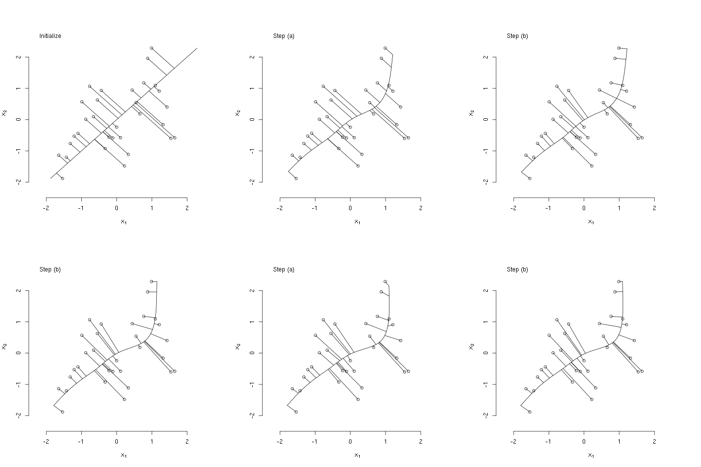
The bit of R code below illustrates the principal curves methods as described in The Elements of Statistical Learning, by Hastie, Tibshirani, and Friedman (Ch. 14; the book is freely available from the authors' website). Specifically, the code generates some bivariate data that have a nonlinear association, initializes the principal curve using the first (linear) principal component, and then computes three iterations of the algorithm described in section 14.5.2. I used the 'animation' package to generate the following animated GIF, which illustrates these steps.
## generate some bivariate data
set.seed(42)
x1 <- seq(1,10,0.3)
w = .6067;
a0 = 1.6345;
a1 = -.6235;
b1 = -1.3501;
a2 = -1.1622;
b2 = -.9443;
x2 = a0 + a1*cos(x1*w) + b1*sin(x1*w) + a2*cos(2*x1*w) +
          b2*sin(2*x1*w) + rnorm(length(x1),0,3/4)
x <- scale(cbind(x1,x2))
alim <- extendrange(x, f=0.1)
alim_ <- range(x)

## plot centered data
plot(x[,1], x[,2], bty='n',
     xlab=expression(x[1]),
     ylab=expression(x[2]),
     xlim=alim, ylim=alim)
legend("topleft", legend=c("Initialize"), bty="n")

## plot first principal component line
svdx <- svd(x)
clip(alim_[1],alim_[2],alim_[1],alim_[2])
with(svdx, abline(a=0, b=v[2,1]/v[1,1]))

## plot projections of each point onto line
z1 <- with(svdx, x%*%v[,1]%*%t(v[,1]))
segments(x0=x[,1],y0=x[,2],
         x1=z1[,1],y1=z1[,2])

## compute initial lambda (arc-lengths associated with
## orthogonal projections of data onto curve)
lam <- with(svdx, as.numeric(u[,1]*d[1]))

for(itr in 1:3) {

  #### step (a) of iterative algorithm ####

  ## compute scatterplot smoother in either dimension
  ## increase 'df' to make the curve more flexible
  fit1 <- smooth.spline(x=lam, y=x[,1], df=4)
  fit2 <- smooth.spline(x=lam, y=x[,2], df=4)

  ## plot data and the principal curve for a sequence of lambdas
  plot(x[,1], x[,2], bty='n',
       xlab=expression(x[1]),
       ylab=expression(x[2]),
       xlim=alim, ylim=alim)
  legend("topleft", legend=c("Step (a)"), bty="n")
  seq_lam <- seq(min(lam),max(lam),length.out=100)
  lines(predict(fit1, seq_lam)$y, predict(fit2, seq_lam)$y)

  ## show points along curve corresponding
  ## to original lambdas
  z1 <- cbind(predict(fit1, lam)$y, predict(fit2, lam)$y)
  segments(x0=x[,1],y0=x[,2],
           x1=z1[,1],y1=z1[,2])


  #### step (b) of iterative algorithm ####

  ## recompute lambdas
  euc_dist <- function(l, x, f1, f2)
    sum((c(predict(f1, l)$y, predict(f2, l)$y) - x)^2)
  lam <- apply(x,1,function(x0) optimize(euc_dist,
    interval=extendrange(lam, f=0.50),
    x=x0, f1=fit1, f2=fit2)$minimum)


  ## show projections associated with recomputed lambdas
  plot(x[,1], x[,2], bty='n',
       xlab=expression(x[1]),
       ylab=expression(x[2]),
       xlim=alim, ylim=alim)
  legend("topleft", legend=c("Step (b)"), bty="n")
  seq_lam <- seq(min(lam),max(lam),length.out=100)
  lines(predict(fit1, seq_lam)$y, predict(fit2, seq_lam)$y)
  z1 <- cbind(predict(fit1, lam)$y, predict(fit2, lam)$y)
  segments(x0=x[,1],y0=x[,2],
           x1=z1[,1],y1=z1[,2])
}
