This semester I'm teaching from Hastie, Tibshirani, and Friedman's book, The Elements of Statistical Learning, 2nd Edition. The authors provide a Mixture Simulation data set that has two continuous predictors and a binary outcome. This data is used to demonstrate classification procedures by plotting classification boundaries in the two predictors. For example, the figure below is a reproduction of Figure 2.5 in the book:
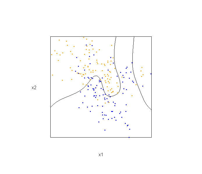
The solid line represents the Bayes decision boundary (i.e., {x: Pr("orange"|x) = 0.5}), which is computed from the model used to simulate these data. The Bayes decision boundary and other boundaries are determined by one or more surfaces (e.g., Pr("orange"|x)), which are generally omitted from the graphics. In class, we decided to use the R package rgl to create a 3D representation of this surface. Below is the code and graphic (well, a 2D projection) associated with the Bayes decision boundary:
library(rgl)
load(url("http://statweb.stanford.edu/~tibs/ElemStatLearn/datasets/ESL.mixture.rda"))
dat <- ESL.mixture


## create 3D graphic, rotate to view 2D x1/x2 projection
par3d(FOV=1,userMatrix=diag(4))
plot3d(dat$xnew[,1], dat$xnew[,2], dat$prob, type="n",
       xlab="x1", ylab="x2", zlab="",
       axes=FALSE, box=TRUE, aspect=1)

## plot points and bounding box
x1r <- range(dat$px1)
x2r <- range(dat$px2)
pts <- plot3d(dat$x[,1], dat$x[,2], 1,
              type="p", radius=0.5, add=TRUE,
              col=ifelse(dat$y, "orange", "blue"))
lns <- lines3d(x1r[c(1,2,2,1,1)], x2r[c(1,1,2,2,1)], 1)

## draw Bayes (True) decision boundary; provided by authors
dat$probm <- with(dat, matrix(prob, length(px1), length(px2)))
dat$cls <- with(dat, contourLines(px1, px2, probm, levels=0.5))
pls <- lapply(dat$cls, function(p) lines3d(p$x, p$y, z=1))

## plot marginal (w.r.t mixture) probability surface and decision plane
sfc <- surface3d(dat$px1, dat$px2, dat$prob, alpha=1.0,
            color="gray", specular="gray")
qds <- quads3d(x1r[c(1,2,2,1)], x2r[c(1,1,2,2)], 0.5, alpha=0.4,
            color="gray", lit=FALSE)
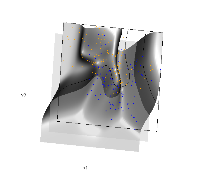
In the above graphic, the probability surface is represented in gray, and the Bayes decision boundary occurs where the plane f(x) = 0.5 (in light gray) intersects with the probability surface.
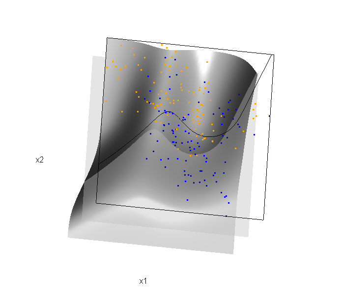
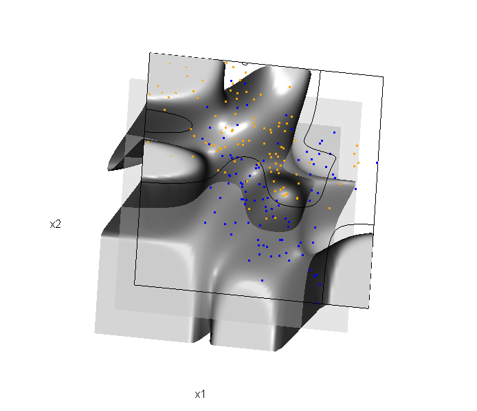
Of course, the classification task is to estimate a decision boundary given the data. Chapter 5 presents two multidimensional splines approaches, in conjunction with binary logistic regression, to estimate a decision boundary. The upper panel of Figure 5.11 in the book shows the decision boundary associated with additive natural cubic splines in x1 and x2 (4 df in each direction; 1+(4-1)+(4-1) = 7 parameters), and the lower panel shows the corresponding tensor product splines (4x4 = 16 parameters), which are much more flexible, of course. The code and graphics below reproduce the decision boundaries shown in Figure 5.11, and additionally illustrate the estimated probability surface (note: this code below should only be executed after the above code, since the 3D graphic is modified, rather than created anew):
Reproducing Figure 5.11 (top):
## clear the surface, decision plane, and decision boundary
par3d(userMatrix=diag(4)); pop3d(id=sfc); pop3d(id=qds)
for(pl in pls) pop3d(id=pl)

## fit additive natural cubic spline model
library(splines)
ddat <- data.frame(y=dat$y, x1=dat$x[,1], x2=dat$x[,2])
form.add <- y ~ ns(x1, df=3)+
                ns(x2, df=3)
fit.add  <- glm(form.add, data=ddat, family=binomial(link="logit"))

## compute probabilities, plot classification boundary
probs.add <- predict(fit.add, type="response",
                     newdata = data.frame(x1=dat$xnew[,1], x2=dat$xnew[,2]))
dat$probm.add <- with(dat, matrix(probs.add, length(px1), length(px2)))
dat$cls.add <- with(dat, contourLines(px1, px2, probm.add, levels=0.5))
pls <- lapply(dat$cls.add, function(p) lines3d(p$x, p$y, z=1))

## plot probability surface and decision plane
sfc <- surface3d(dat$px1, dat$px2, probs.add, alpha=1.0,
                 color="gray", specular="gray")
qds <- quads3d(x1r[c(1,2,2,1)], x2r[c(1,1,2,2)], 0.5, alpha=0.4,
               color="gray", lit=FALSE)
Reproducing Figure 5.11 (bottom)
## clear the surface, decision plane, and decision boundary
par3d(userMatrix=diag(4)); pop3d(id=sfc); pop3d(id=qds)
for(pl in pls) pop3d(id=pl)

## fit tensor product natural cubic spline model
form.tpr <- y ~ 0 + ns(x1, df=4, intercept=TRUE):
                    ns(x2, df=4, intercept=TRUE)
fit.tpr  <- glm(form.tpr, data=ddat, family=binomial(link="logit"))

## compute probabilities, plot classification boundary
probs.tpr <- predict(fit.tpr, type="response",
                     newdata = data.frame(x1=dat$xnew[,1], x2=dat$xnew[,2]))
dat$probm.tpr <- with(dat, matrix(probs.tpr, length(px1), length(px2)))
dat$cls.tpr <- with(dat, contourLines(px1, px2, probm.tpr, levels=0.5))
pls <- lapply(dat$cls.tpr, function(p) lines3d(p$x, p$y, z=1))

## plot probability surface and decision plane
sfc <- surface3d(dat$px1, dat$px2, probs.tpr, alpha=1.0,
                 color="gray", specular="gray")
qds <- quads3d(x1r[c(1,2,2,1)], x2r[c(1,1,2,2)], 0.5, alpha=0.4,
               color="gray", lit=FALSE)
Although the graphics above are static, it is possible to embed an interactive 3D version within a web page (e.g., see the rgl vignette; best with Google Chrome), using the rgl function writeWebGL. I gave up on trying to embed such a graphic into this WordPress blog post, but I have created a separate page for the interactive 3D version of Figure 5.11b. Duncan Murdoch's work with this package is really nice!
Honestly i don't see why 3D adds anything here. Cool it can be done though
Yes, I showed these to one of my colleagues and he said the same thing; that he didn't feel that the added information in these graphics was particularly helpful. I agree to some extent, but I found the irregularity of the surface associated with the tensor product splines a bit surprising. We made similar 3D graphics for the LDA and QDA decision boundaries (e.g., Figure 4.1 from the book), and found that much more useful.
Well, I think it at least has a great educational value. An excellent post - thanks for sahring.
Jaroslaw Piskorski