That's a mouthful! I presented this topic to a group of Vandy statisticians a few days ago. My notes (essentially reproduced in this post) are recorded at the Dept. of Biostatistics wiki: HowToBootstrapCorrelatedData. The presentation covers some bootstrap strategies for hierarchically structured (correlated) data, but focuses on the multi-stage bootstrap; an extension of that described by Davison and Hinkley (ISBN 978-0-521-57471-6).
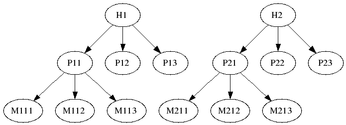
The multi-stage bootstrap mimics the data generating mechanism by resampling in a nested fashion. For example, resample first among factors at the highest level of hierarchy. Then, for each resampled factor, further resample among factors at the next lower level, and so forth. Each level may be resampled with or without replacement. Furthermore, some levels of hierarchy may be ignored completely, if considered to have little or no effect on the data correlation structure. Whether to ignore a level of hierarchy, or to sample with replacement are important bootstrap design considerations.
The resample function below implements a multi-stage bootstrap recursively. That is, levels of hierarchy are traversed by nested calls to resample. The dat argument is a dataframe with factor fields for each level of hierarchy (e.g., hospital, patient, measurement), and a numeric field of measured values. The cluster argument is a character vector that identifies the hierarchy in order from top to bottom (e.g., c('hospital','patient','measurement')). The replace argument is a logical vector that indicates whether sampling should be with replacement at the corresponding level of hierarchy (e.g., c(TRUE,FALSE,FALSE)).
resample <- function(dat, cluster, replace) {

  # exit early for trivial data
  if(nrow(dat) == 1 || all(replace==FALSE))
      return(dat)

  # sample the clustering factor
  cls <- sample(unique(dat[[cluster[1]]]), replace=replace[1])

  # subset on the sampled clustering factors
  sub <- lapply(cls, function(b) subset(dat, dat[[cluster[1]]]==b))

  # sample lower levels of hierarchy (if any)
  if(length(cluster) > 1)
    sub <- lapply(sub, resample, cluster=cluster[-1], replace=replace[-1])

  # join and return samples
  do.call(rbind, sub)

}
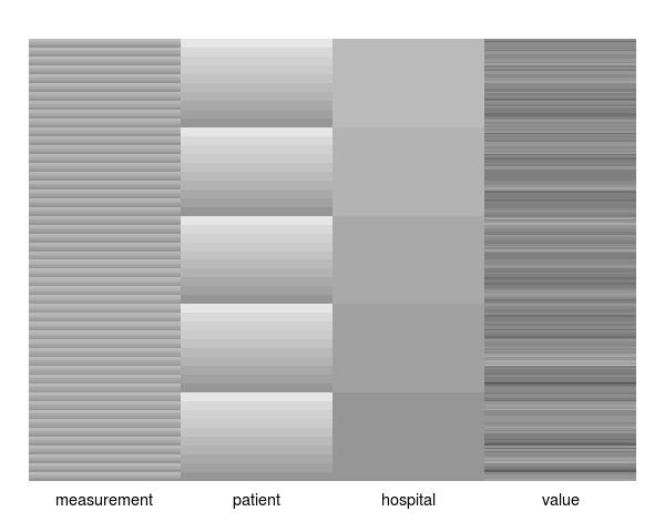
The following block of R code simulates a dataset with 5 correlated (rho = 0.4) repeat measurements on each of 10 patients, from each of 5 hospitals. Hence, there are 250 simulated measurements and 50 patients in total. Patients are simulated independently (i.e., the hospital level of hierarchy has no affect on the correlation structure). The functions covimage and datimage generate a levelplot representations of the covariance and data matrices for the simulated data, respectively.
# simulate correlated data
rho <- 0.4
dat <- expand.grid(
  measurement=factor(1:5),
  patient=factor(1:10),
  hospital=factor(1:5))
sig <- rho * tcrossprod(model.matrix(~ 0 + patient:hospital, dat))
diag(sig) <- 1
dat$value <- chol(sig) %*% rnorm(250, 0, 1)

library("lattice")

covimage <- function(x)
   levelplot(as.matrix(x), aspect="fill", scales=list(draw=FALSE),
      xlab="", ylab="", colorkey=FALSE, col.regions=rev(gray.colors(100, end=1.0)),
      par.settings=list(axis.line=list(col=NA,lty=1,lwd=1)))

datimage <- function(x) {
   mat <- as.data.frame(lapply(x, as.numeric))
   levelplot(t(as.matrix(mat)), aspect="fill", scales=list(cex=1.2, y=list(draw=FALSE)),
      ylab="", xlab="", colorkey=FALSE, col.regions=gray.colors(100),
      par.settings=list(axis.line=list(col=NA,lty=1,lwd=1)))
}

datimage(dat)
covimage(sig)
The images below result from calls to datimage(dat) and covimage(dat) respectively.
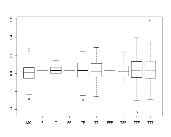
The next block of R code generates several boostrap distributions for the sample mean, and approximates the 'true' sampling distribution by Monte Carlo. The final series of boxplots (shown below) illustrate that bootstrap design greatly impacts the inferred distribution of the sample mean (and presumably for other sample statistics). Hence, it's important to think carefully about bootstrap design for hierarchically structured data, and ensure that it closely reflects the 'true' data generating mechanism.
# bootstrap ignoring hospital and patient levels
cluster <- c("measurement")
system.time(mF <- replicate(200, mean(resample(dat, cluster, c(F))$val)))
system.time(mT <- replicate(200, mean(resample(dat, cluster, c(T))$val)))
#boxplot(list("F" = mF, "T" = mT))

# bootstrap ignoring hospital level
cluster <- c("patient","measurement")
system.time(mFF <- replicate(200, mean(resample(dat, cluster, c(F,F))$val)))
system.time(mTF <- replicate(200, mean(resample(dat, cluster, c(T,F))$val)))
system.time(mTT <- replicate(200, mean(resample(dat, cluster, c(T,T))$val)))
#boxplot(list("FF" = mFF, "TF" = mTF, "TT" = mTT))

# bootstrap accounting for full hierarchy
cluster <- c("hospital","patient","measurement")
system.time(mFFF <- replicate(200, mean(resample(dat, cluster, c(F,F,F))$val)))
system.time(mTFF <- replicate(200, mean(resample(dat, cluster, c(T,F,F))$val)))
system.time(mTTF <- replicate(200, mean(resample(dat, cluster, c(T,T,F))$val)))
system.time(mTTT <- replicate(200, mean(resample(dat, cluster, c(T,T,T))$val)))
#boxplot(list("FFF" = mFFF, "TFF" = mTFF, "TTF" = mTTF, "TTT" = mTTT))

# Monte Carlo for the true sampling distribution
system.time(mMC <- replicate(200, mean(chol(sig) %*% rnorm(250, 0, 1))))
#boxplot(list("MC" = mMC))

boxplot(list("MC" = mMC,
             "F" = mF, "T" = mT,
             "FF" = mFF, "TF" = mTF, "TT" = mTT,
             "FFF" = mFFF, "TFF" = mTFF, "TTF" = mTTF, "TTT" = mTTT))
The following figure presents boxplots for the distribution of sample means under the above sequence of bootstrap strategies. The "MC" boxplot summarizes the 'true' distribution of the sample mean (estimated using Monte Carlo). The remaining boxplots are labeled according to the bootstrap strategy used. For instance, the "TF" boxplot corresponds to a multi-stage bootstrap of patients with replacement and measurements-within-patients without replacement (this is commonly called the "cluster bootstrap"), but that ignores the hospital factor. This strategy most closely reflects the data generating mechanism. Notice that sampling all levels of hierarchy without replacement (e.g., "FFF") simply permutes the indices of the resampled data, and does not confer any variability on the sample mean.


